Excel Formulas Not Working? Ways to Fix Them

Stuck staring at error messages instead of getting results? You’re not alone. Excel formulas are powerful, but they can be finicky. Don’t panic! This guide will walk you through common fixes to get your formulas working smoothly and your spreadsheets singing.

In this article, I’ll share my tried-and-true methods for troubleshooting and resolving formula errors in Excel. Whether you’re a beginner or an advanced user, these tips will help you optimize your spreadsheets and avoid formula errors in the future.

Common Formula Errors in Excel

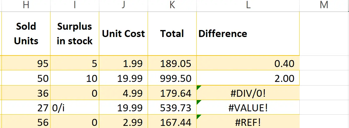
One of the most frustrating experiences for an Excel user is encountering a formula error. Despite your best efforts to input the correct formula, Excel just won’t compute the results you’re looking for. Here are the most popular formula errors:

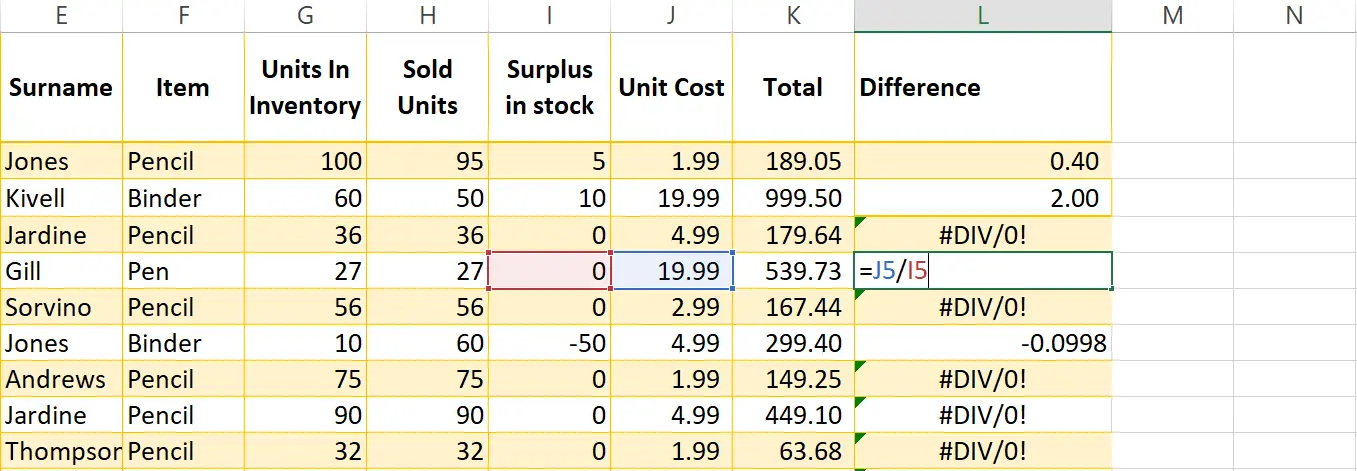
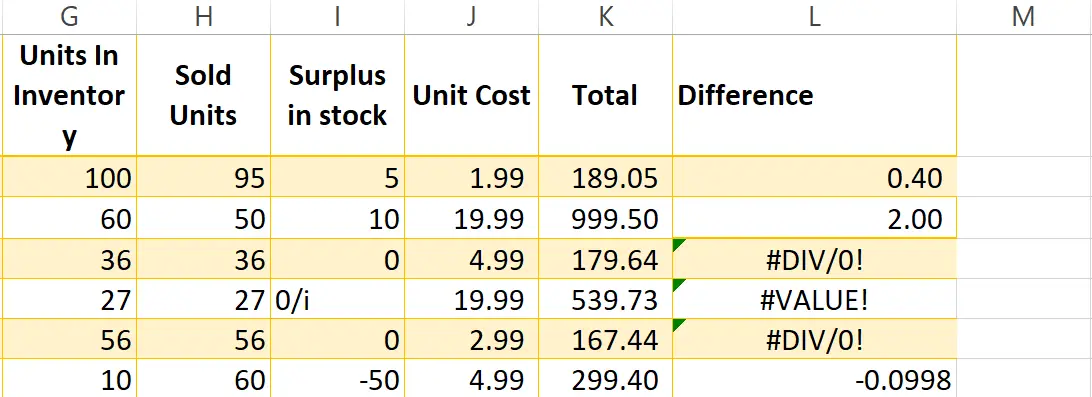
#DIV/0! Error

The #DIV/0! error in Excel shows up when you try to divide by zero.

Here’s how to fix it:

1. Check for Zeros and Blank Cells: Make sure the cell you’re dividing by isn’t zero or blank. Fix any data entry mistakes.
2. Use IF Function: Use the IF function to handle potential zeros. For example, =IF(B2=0, "Error", A1/B2) displays “Error” if cell B2 is zero, otherwise it shows the original formula result.
3. Change Cell Reference: If the error comes from another formula, adjust the cell reference to avoid dividing by zero.

#VALUE! Error:

The #VALUE! error in Excel indicates a mismatch between the data type you’re using and the operation you’re trying to perform.

Here are some common causes and solutions:

• Text vs. Numbers: Excel might interpret your data as text instead of numbers. Try removing leading or trailing spaces from cells. You can also use functions like VALUE or CLEAN to convert text to numbers.
• Incorrect Formula Syntax: Double-check your formula for typos or misplaced parentheses. Excel is very particular about syntax.
• Invalid References: Make sure the cells you’re referencing in your formula actually contain data and are spelled correctly.
• Dates as Text: If you’re trying to perform calculations on dates formatted as text, Excel will throw a #VALUE! error. Convert them to a proper date format using the DATE function.
• Logical Errors: Sometimes the formula itself might be logicaly flawed. For instance, trying to take the square root of a negative number.

Related Article: How To Analyze Data In Excel Spreadsheet

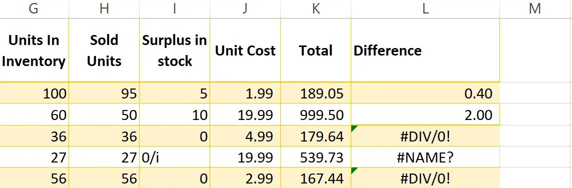
#NAME? Error:

The #NAME? error in Excel pops up when it can’t recognize something in your formula.

Here’s how to tackle it:

1. Misspelled Formula Name: This is a common culprit. Double-check that you’ve spelled the function name correctly. Excel is case-sensitive, so SUM and sum are not the same!
2. Missing Quotes: If you’re using text within your formula, make sure it’s enclosed in double quotes (“”). Otherwise, Excel might misinterpret it as a function or named range.
3. Incorrect Named Range: If your formula references a named range (a custom cell or range name), ensure it’s spelled correctly and refers to a valid range.
4. Scope Issues: Named ranges can be sheet-specific. If the named range is on a different sheet than your formula, you might need to adjust the reference to include the sheet name (e.g., Sheet1!MyRange).

#REF! Error:

The #REF! error in Excel shows up when a formula references a cell or range that Excel can’t find.

Here’s how to get your formulas back on track:

1. Deleted Cells or Ranges: Did you delete rows, columns, or entire sheets that were referenced in your formulas? Excel can’t find those references anymore. Adjust the formulas to point to valid locations.
2. Incorrect Cell References: Double-check that you haven’t mistyped cell references in your formulas. A simple typo can cause this error.
3. Relative vs. Absolute References: Are you using relative references (A1) that change when copied, or absolute references ($A$1) that stay fixed? Ensure your references are correct for the formula’s location.
4. Hidden Rows or Columns: If the referenced cells are hidden, Excel won’t recognize them. Unhide rows or columns to resolve the error.
5. External References: Are your formulas referencing cells in a different workbook that’s not open? Ensure both workbooks are open and the reference path is correct.

Here are some additional tips:

• Use the Find and Replace function (Ctrl+F) to search for all #REF! errors in your worksheet.
• Consider using absolute references or named ranges to make your formulas more robust against changes in your spreadsheet.

Related article: 7 Best AI For Data Analysis: Tools You Can’t Miss

How To Generate Formulas With AI? To Avoid Errors

AI is stepping up to make spreadsheet life easier. New tools can now generate formulas based on your descriptions, helping you avoid errors and write formulas faster. Here’s a step-by-step guide to get started:

1. Create a free Ajelix account

Simplify your spreadsheets with Ajelix, an AI platform offering over 15 tools including an Excel formula generator. Sign up easily using your Gmail or any email address.

Screenshot from Ajelix registration page, image by author

2. Locate the Formula generator tool

After logging into the Ajelix portal, head to the AI tools section to find the Excel formula generator.

Screenshot from Ajelix portal on how to find formula generator, image by author

3. Write a clear and concise prompt

The best way to get the right formula is to clearly explain what you’re trying to calculate. Be specific! For instance, instead of just saying ‘Give me the NPV formula,’ you could say ‘What’s the formula for Net Present Value (NPV) if my cash flows are in cells B2:B7 and my discount rate is 10 percent?’

Screenshot from Ajelix formula generator with NPV prompt, image by author

Crafting Powerful Prompts for Formulas:

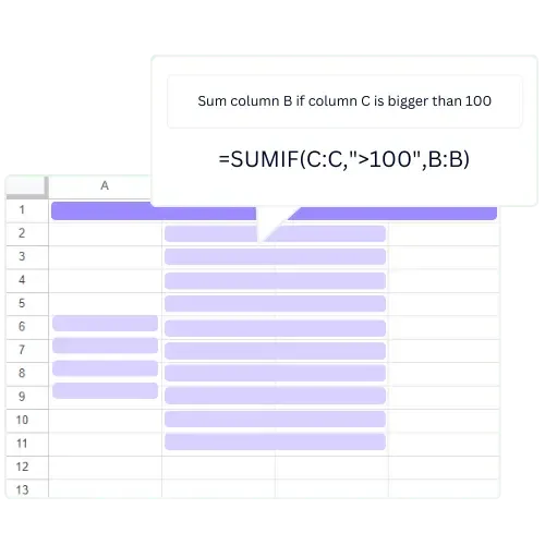
• Define Your Goal: Instead of a vague request for a formula, state the specific calculation you need. Aim for clarity, like: “Calculate the average sales in column B for items marked ‘Yes’ in column A.”
• Use Cell References: If your program allows, include specific cell or range names. This improves accuracy: “Calculate the total cost (column C) by multiplying quantity (column A) by price (column B).”
• Specify Conditions Clearly: When your formula involves conditions, explain them precisely. For example: “Return ‘Bonus’ in cell D2 if sales (column B2) exceed target (cell E1), otherwise return ‘No Bonus’.”

4. Get your formula

Once you have the prompt AI will give you a ready-to-use formula to insert in your spreadsheet. You can also use Excel or Google Sheets add-on for easier formula writing.

In the answer below you can see that AI gave the correct formula and in the FAQ wrote additional tips to create a correct formula. You can also see common mistakes, which helps you avoid further errors.

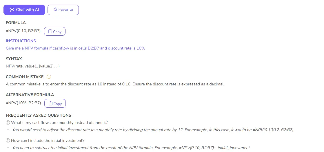
Screenshot from Ajelix with NPV formula result, image by author

Common Excel Formula Mistakes and Fixes

Function	Mistake	Fix
All Functions	#####	Widen the column to display the full formula result.
All Functions	#NAME?	Check for typos in the function name or cell references.
SUM	Incorrect range selection	Ensure you’ve selected the entire range of cells to sum (including empty cells).
SUM	Text in cells	Format the cells as numbers or remove text before summing.
VLOOKUP	Typos in cell references	Double-check the spelling of sheet and cell names used in the formula.
VLOOKUP	Incorrect lookup criteria	Make sure your lookup value exactly matches the criteria in the table.
IF	Syntax errors	Ensure correct use of symbols (=, <>, <> ) and parentheses.
IF	Logical errors	Verify your IF condition accurately reflects what you want to test (e.g., =A1>10, not >A10).
IF	Missing results	Define what to show for both TRUE and FALSE outcomes (e.g., “Yes”, “No”).
Sheet References	Typos in sheet name	Double-check for typos in the sheet name referenced in the formula.
Sheet References	Hidden sheet	Ensure the referenced sheet is visible and not hidden.
Sheet References	Missing cell	Verify the referenced cell exists in the other sheet (avoid referencing deleted rows/columns).
AVERAGE	Empty cells	Excludes empty cells by default. Use AVERAGEA to include them.
COUNTIF	Incorrect criteria	Ensure your criteria accurately reflects what you want to count (e.g., “>10”, not =”>10”).
COUNTIFS	Multiple criteria issues	Double-check the range and criteria for each condition in the function.
FIND	Case sensitivity	FIND is case-sensitive. Use FIND.B to ignore case.
MATCH	Not finding exact match	Use EXACT function within MATCH for exact matches.

Related article: Collaborative Business Intelligence (BI) & Analytics

Auditing Tools: For Excel Formulas Not Working Issues

As we’ve discussed, encountering formula errors in Excel can be a frustrating experience. However, with Excel’s built-in formula auditing tools, troubleshooting and resolving these errors has never been easier. In this section, we’ll discuss some of the most helpful formula auditing tools and how to use them.

Trace Dependents

The Trace Dependents tool allows you to see which cells are dependent on a particular formula. To use this tool, simply select the cell with the formula you want to check and click the “Trace Dependents” button in the “Formula Auditing” section of the “Formulas” tab. Excel will then highlight all cells that depend on the selected cell.

Trace Precedents

The Trace Precedents tool works in reverse to the Trace Dependents tool. It allows you to see which cells a particular formula is dependent on. To use this tool, select the cell with the formula you want to check and click the “Trace Precedents” button in the “Formula Auditing” section of the “Formulas” tab. Excel will then highlight all cells that the selected cell depends on.

Evaluate Formula

The Evaluate Formula tool allows you to step through a complex formula and see the intermediate results at each stage of the calculation. To use this tool, select the cell with the formula you want to check and click the “Evaluate Formula” button in the “Formula Auditing” section of the “Formulas” tab. Excel will then step through the formula and show you the intermediate results at each stage.

By using these formula auditing tools, you can quickly and easily identify and resolve formula errors in Excel. In the next section, we’ll discuss some additional tips and best practices for avoiding formula errors in the first place.

Related article: How To Add Drop Down List in Excel

Check for Syntax Errors: Catch Mistakes Before They Happen

While Excel’s formula auditing tools are invaluable for troubleshooting errors, it’s even better to catch mistakes before they happen. One of the best ways to do this is by checking your formulas for syntax errors.

Check Parentheses

One of the most common syntax errors in Excel formulas is mismatched or missing parentheses. To catch these errors, always double-check that your parentheses are balanced and match each other.

Check Operators

Another common syntax error is using the wrong operator in your formula. For example, if you’re trying to multiply two cells together, but accidentally use the division operator, your formula won’t work as expected. Always double-check that you’re using the correct operators in your formulas.

Check Cell References

A third common syntax error is referencing the wrong cells in your formulas. This can happen if you accidentally delete or move a cell that is referenced in your formula. Always double-check that your cell references are accurate and up-to-date.

Use the Formula Bar

The Formula Bar in Excel is a powerful tool for checking your formulas for syntax errors. Whenever you’re working on a formula, make sure to double-check it in the Formula Bar before pressing enter. This will allow you to catch any syntax errors before they cause problems.

By checking your formulas for syntax errors, you can catch mistakes before they happen and save yourself a lot of time and frustration in the long run.

Ensure Data Types Match: Avoid Common Calculation Errors

In addition to syntax errors, another common source of Excel formula errors is data type mismatches. When you’re working with formulas in Excel, it’s important to ensure that your data types match to avoid common calculation errors. In this section, we’ll discuss some tips and best practices for ensuring that your data types match in Excel.

Understand Data Types

Before you can ensure that your data types match, you need to understand the different types of data that Excel supports. These include text, numbers, dates, times, and Boolean values (TRUE or FALSE). Make sure you understand the data types you’re working with and how they interact with each other in Excel formulas.

Use Data Validation

Excel’s Data Validation feature is a powerful tool for ensuring that your data types match. By setting up data validation rules, you can prevent users from entering data that doesn’t match the expected data type. For example, you can set up a rule that only allows users to enter dates in a particular format.

Use Functions to Convert Data Types

If you’re working with data that’s in the wrong format, you can use Excel’s built-in functions to convert it to the correct data type. For example, you can use the DATEVALUE function to convert a text string that represents a date into an actual date value that Excel can work with.

Pay Attention to Calculation Results

Finally, always pay attention to the results of your calculations in Excel. If you’re getting unexpected results, it could be a sign that your data types are mismatched. Double-check your formulas and make sure that your data types match.

By following these tips and best practices, you can avoid common calculation errors in Excel and ensure that your formulas are working correctly. In the next section, we’ll provide you with best practices on using named ranges to avoid errors.

Related article: Data Visualization For Small Business: Where To Start?

Use Named Ranges: Make Your Formulas Easier to Understand and Maintain

If you’re working with complex formulas in Excel, you may find that it’s difficult to keep track of all the cell references. This is where named ranges come in handy. By using named ranges, you can make your formulas easier to understand and maintain. In this section, we’ll discuss some tips and best practices for using named ranges in Excel.

What Are Named Ranges?

A named range is a descriptive name that you give to a cell or range of cells in Excel. Instead of using cell references in your formulas, you can use the named range instead. This makes your formulas easier to read and understand and also makes them more flexible and easier to maintain.

Create Meaningful Names

When you’re creating named ranges in Excel, it’s important to use meaningful names that describe the data you’re working with. For example, instead of using “A1:B10” to refer to a range of sales data, you could create a named range called “SalesData”.

Use Relative or Absolute References

When you create a named range in Excel, you can choose to use either relative or absolute references. Relative references are based on the position of the named range relative to the cell that contains the formula. Absolute references are fixed and don’t change if you move the named range. Choose the type of reference that makes the most sense for your data and formulas.

Organize Your Named Ranges To Avoid Formulas Not Working

If you’re working with a lot of named ranges in Excel, it’s important to keep them organized. You can do this by grouping them together in a separate worksheet, or by using a naming convention that makes it easy to find and identify your named ranges.

By using named ranges in your Excel formulas, you can make your formulas easier to understand and maintain. In the final section of this article, we’ll summarize the key takeaways and provide some additional resources for mastering Excel formulas.

Related article: Free Break-Even Point Calculator Online

Avoid Circular References: Keep Your Formulas Running Smoothly

One of the most common Excel formula errors is the circular reference error. This occurs when a formula refers back to the cell that it’s located in, creating a circular reference that Excel can’t resolve. In this final section, we’ll discuss some tips and best practices for avoiding circular references in your Excel formulas.

Understand Circular References

Before you can avoid circular references in Excel, you need to understand what they are and how they occur. A circular reference occurs when a formula refers back to the cell where it’s located. For example, if you enter “=A1+A2” in cell A1, and “=A1+10” in cell A2, you’ll have a circular reference.

Use Iterative Calculation

One way to avoid circular references in Excel is to use iterative calculation. Iterative calculation is a setting in Excel that allows a formula to refer back to the cell it’s located in, as long as the formula is set up to handle circular references correctly. You can turn on iterative calculation in the Excel Options menu.

Break Circular References

If you do have a circular reference in your Excel formula, you can break it by changing the formula to refer to a different cell. For example, if you have a formula in cell A1 that refers to cell A1, you can change it to refer to cell A2 instead.

Use Formulas with Care

Finally, always use formulas with care in Excel. If you’re not sure how a formula will behave, test it in a separate worksheet before using it in your actual data. And always double-check your formulas for circular references and other errors.

By following these tips and best practices, you can avoid circular reference errors in Excel and keep your formulas running smoothly. With a little practice and attention to detail, you can become a master of Excel formulas and take your data analysis skills to the next level.

Related article: How To Build AI Dashboard For Data Analytics Tasks

Conclusion Why Formulas Not Working and How To Fix That

In summary, we’ve covered several ways to fix Excel formula errors including identifying common errors, using formula auditing tools, checking for syntax errors, ensuring data types match, using named ranges, and avoiding circular references. By applying these tips, you can avoid common pitfalls and make the most of Excel’s powerful formula capabilities.

Learn more about Excel and Google Sheets hacks in other articles. Stay connected with us on social media and receive more daily tips and updates.

FAQ