From data to report in one minute or less. Ajelix BI is launched! 🚀 Get started for free.

How To Use SKEW function in Excel With Examples

What is SKEW function in Excel?

SKEW function in Excel calculates the standard deviation of the logarithms of the individual values in a data set. The Excel function helps you understand your data’s distribution and identify potential outliers.

Description

The SKEW function in Excel is used to calculate the skewness of a data set. Skewness is a measure of the asymmetry of a probability distribution. It measures how far a set of numbers is spread out from its average. Positive skewness indicates a distribution with an asymmetric tail extending toward more positive values. Negative skewness indicates an asymmetric tail extending toward more negative values.

The function calculates the skewness of a data set based on the formula given by the moment coefficient of skewness. The function takes an array of numbers or a range of cells containing numbers as its argument. It will then return the skewness of the data set as a decimal number. A number close to zero indicates a normal distribution, while higher and lower numbers indicate more positive or negative skewness respectively.

The SKEW formula can quickly identify if a data set is symmetrical or asymmetrical. It can also help to identify the direction of an asymmetry and can be used to compare the skewness of different data sets. The function can be used for fundamental analysis of data sets, for example, to identify potential outliers. It is also an important part of more complex statistical calculations, such as finding the kurtosis of a data set.

Struggling with your Excel formulas?
Looking for a faster and easier way to write Excel formulas? Try AI Excel Formula Generator and turn your text into formulas with just a few clicks.

Try for free

Syntax

=SKEW(number1, [number2], …)

Where number1, number2, etc. are the numbers or cell references for which you want to calculate the skewness.

How To Generate Formulas With AI?

Unlock new possibilities in your spreadsheets! This guide explores how AI can help you work more efficiently with data.

1. Create a free Ajelix account

Explore Ajelix for efficient spreadsheets! This platform offers over 15 AI tools, including Excel formula generator, to help you automate tasks and manage complex spreadsheets. Sign up easily with Gmail or any email address to discover its functionalities.

Register on ajelix.com and create a free account to generate formulas screenshot from platform

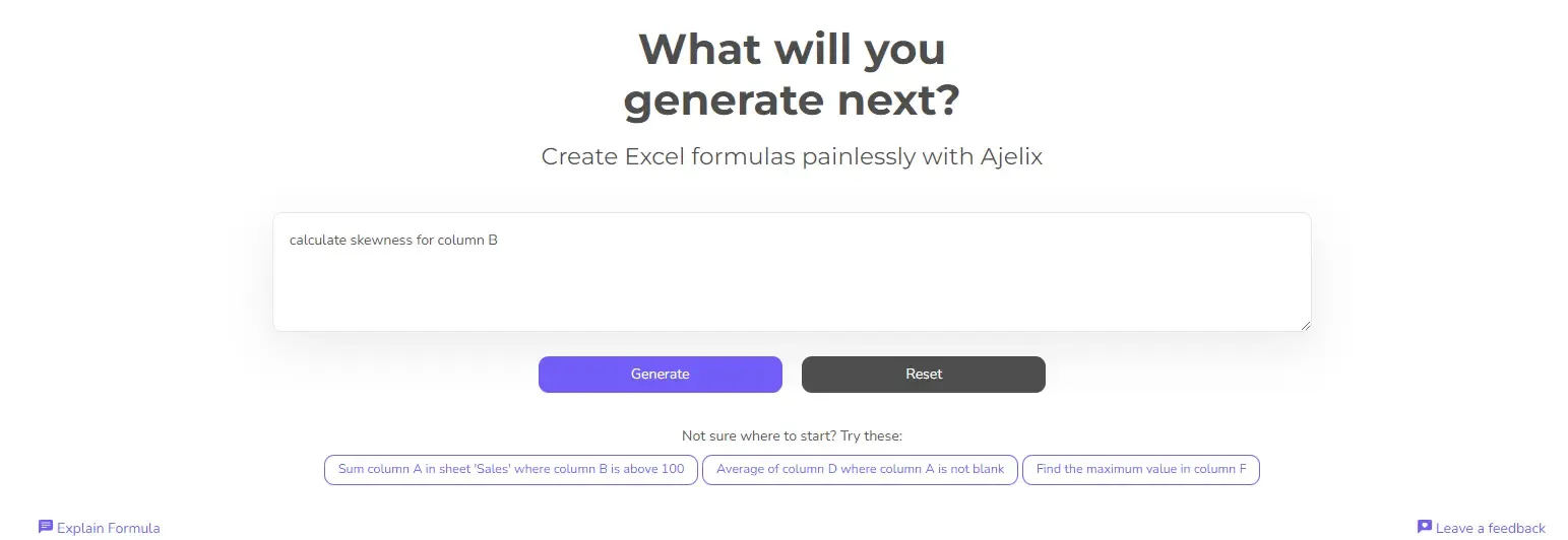
2. Write a concise prompt

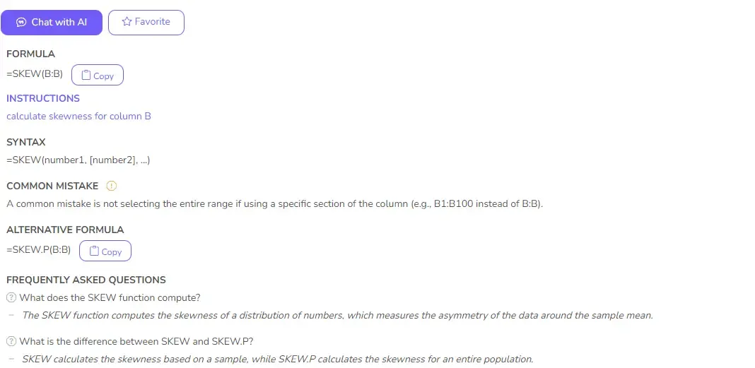
The secret to a perfect formula? Clear communication! Instead of focusing on specific functions, tell the AI what you want to calculate in plain language. For example, to get the SKEW formula, say: “Calculate skewness for column B” The clearer you explain your goal, the better the AI can understand your needs and provide the right formula.

skew function prompt for AI screenshot from portal with prompt

3. Get Your Formula

Craft your request, get your formula, and breeze through spreadsheets! The AI will analyze your description and provide a ready-made formula you can simply copy and paste into your spreadsheet for immediate use. Want an even smoother workflow? Explore Excel or Google Sheets add-ons built specifically for AI formula generation. (See the example below for an AI-powered formula that tackles your needs precisely.

SKEW formula result from AI screenshot from portal with function

Ready to give it a go?
Test AI tools with freemium plan and only upgrade if formula generator can help you!

Give it a go

SKEW Function MS Excel - Ajelix Excel Formulas Cheat Sheet

How to use Excel SKEW function in your workbook:

  1. Open the Excel file containing the data set that you want to skew.
  2. Select the data set and click on the Insert tab.
  3. In the Charts group, click on the Line chart icon.
  4. Choose the “skew” option from the drop-down menu.
  5. The skewed chart will automatically be generated in the same worksheet.
  6. To adjust the skew amount, right-click on the chart and select “Format Data Series”.
  7. In the Format Data Series window, select the “Skew” tab and adjust the skew accordingly.
  8. Click OK to apply the changes.
  9. To further customize your chart, use the Chart Tools tab.
  10. Select the Design tab and choose from a variety of customization options.
  11. To finish, click the Save icon to save the chart.

Frequently Asked Questions

What does a positive or negative skewness value mean?

A positive skewness value indicates that the data distribution has a longer tail to the right (positive skew) or more values above the mean, while a negative skewness value indicates a longer tail to the left (negative skew) or more values below the mean. A skewness value of 0 means the data is perfectly symmetrical.

Can the SKEW function return an error?

Yes, the SKEW function can return the #DIV/0! error if the standard deviation of the data is equal to zero, which means there is no variation and the skewness cannot be calculated. The function can also return the #VALUE! error if the supplied range contains non-numeric values.

Can the SKEW formula be used with non-contiguous ranges?

Yes, the SKEW function can be used with non-contiguous ranges by using multiple range references separated by a comma within the function’s argument. However, each range must be enclosed in parentheses and the total number of values cannot exceed the maximum allowed by Excel.

Excel guides

Calculators

Analytics & Business Intelligence