Excel Statistical Functions with Examples

Good old Excel with its wide range of statistical functions is a powerhouse when it comes to data analysis. Whether you are a beginner or an experienced user, knowing how to use Excel Statistical Functions can make your data analysis process more efficient and accurate.
Let’s dive in and explore some of the most commonly used Excel Statistical Functions with Examples.
AVERAGE Function
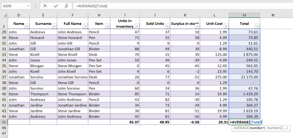
The AVERAGE function calculates the arithmetic mean of a range of numbers.
This might interest you: How to use the AVERAGE Function
For example, if you want to find the average of a set of numbers (10, 20, 30), you can use the formula =AVERAGE(10, 20, 30), or =AVERAGE(M1:M44) if the numbers are in a range of cells. Take a look at our example below.
COUNT Function
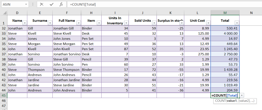
The COUNT function is used to count the number of cells in a range that contain numbers. For example, if you have a range of numbers (10, 20, 30, and a blank cell), the formula =COUNT(M1:M44) will return the value 43, which is the number of cells containing numbers.
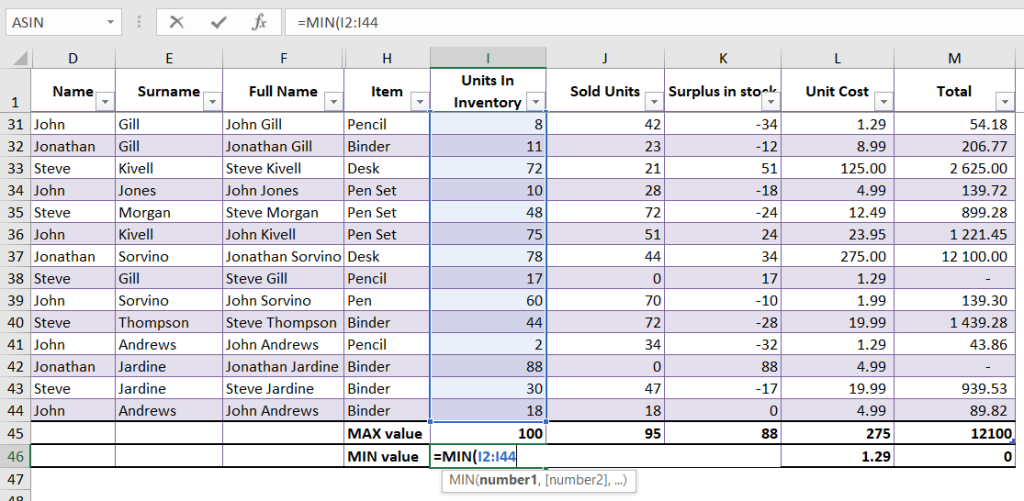
MAX and MIN Functions
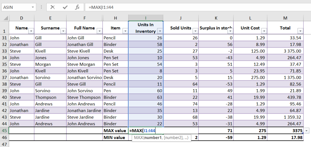
The MAX and MIN functions are used to find the highest and lowest values in a range of numbers. We have created a separate guide for each function, where you can read more about MAX and MIN functions.
For example, if you have a range of numbers (10, 20, 30), the formula =MAX(I1:I44) will return 100, and the formula =MIN(I1:I44) will return 10.
Our Free Excel Formula & Script library might interest you.
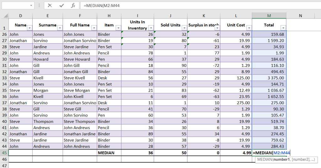
MEDIAN Function
Use the MEDIAN function to find the middle value in a range of numbers. We have also created a guide for this function.
For example, if you have a range of numbers (10, 20, 30, 40), the formula =MEDIAN(A1:D1) will return 25, which is the middle value.
Statistical Functions: MODE Function
The MODE function finds the most frequently occurring value in a range of numbers. For example, if you have a range of numbers (10, 20, 20, 30, 30), the formula =MODE(A1:E1) will return 20 and 30, which are the most frequently occurring values.
STDEV.P and STDEV.S Functions
The STDEV.P and STDEV.S functions are used to calculate the standard deviation of a range of numbers.
This might interest you: How to use the STDEV Function
The STDEV.P function is used for a population, while the STDEV.S function is used for a sample. For example, if you have a range of numbers (10, 20, 30, 40), the formula =STDEV.P(A1:D1) will return the population standard deviation, and the formula =STDEV.S(A1:D1) will return the sample standard deviation.
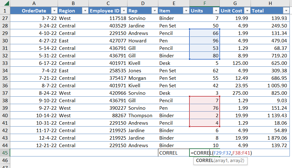
CORREL Function
The CORREL function is used to find the correlation coefficient between two sets of data.
This might interest you: How to use the CORREL Function
For example, if you have two sets of data (A1:A5 and B1:B5), the formula =CORREL(A1:A5, B1:B5) will return the correlation coefficient between the two sets of data. The correlation coefficient ranges from -1 to 1, where -1 indicates a perfect negative correlation, 0 indicates no correlation, and 1 indicates a perfect positive correlation.
Statistical Functions: TREND Function
The TREND function is used to predict future values based on a linear trend. For example, if you have a set of data (A1:A5 and B1:B5), you can use the formula =TREND(B1:B5, A1:A5). This function is useful for forecasting trends and making data-driven predictions.
FREQUENCY Function
The FREQUENCY function is used to count the number of values within a range that fall into specified intervals. For example, if you have a range of numbers (10, 20, 30, 40, 50) and you want to count the number of values that fall between 20 and 40, you can use the formula =FREQUENCY(A1:E1, {0,20,40,60}).
This will return an array of values, with the first value indicating the number of values less than 20. The second value indicates the number of values between 20 and 40. The third value indicates the number of values between 40 and 60.
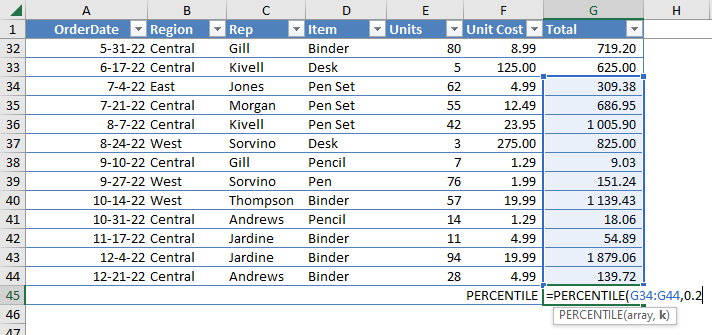
Statistical Functions: PERCENTILE Function
Use the PERCENTILE function to find the nth percentile of a range of values. For example, if you have a range of numbers (10, 20, 30, 40, 50) and you want to find the 70th percentile, you can use the formula =PERCENTILE(G34:G44, 0.7). This will return the value 38, which is the value that is greater than or equal to 70% of the values in the range.
Conclusion
Happy Excel-ing! With these Excel Statistical Functions, you can gain valuable insights into your data and make better decisions based on the results of your analysis. With a little practice and experimentation, you can become proficient.
In case you want to learn more, Microsoft has made a summary of statistical functions.
Don’t hesitate to reach out to us for any further guidance or queries related to Excel statistical functions.
It’s also ok to feel like Garfield sometimes, so feel free to give AI the annoying task of generating Excel Formulas and try Excel Formula Generator for free!
Want to stay in the tips and tricks loop? Sure, let’s stay connected.
FAQ
Statistical functions in Excel help analyze numerical data by calculating averages, frequencies, correlations, percentiles, and other statistical measures. For example, functions, like AVERAGE, COUNT, MODE, STDEV, and PERCENTILE, are statistical.
The AVERAGE function calculates the arithmetic mean of a range of numbers. For example, =AVERAGE (10,20,30) returns 20.
STDEV.P calculates the standard deviation for an entire population, while STDEV.S is used for a sample.
You can use the MODE function. For example, =MODE(A1:10) returns the most common number in the range.
Speed up your spreadsheet tasks with Ajelix AI in Excel