SLOPE function MS Excel

SLOPE Function in Excel calculates the slope of a line when given two points on that line. It returns the slope of the linear regression line that best fits the data points using the least squares method. 

The SLOPE function in Excel is a useful tool for analyzing the relationship between two variables. It allows you to calculate the slope of a line based on two sets of coordinates, making it easy to determine the rate of change between the variables. This function can be especially helpful in trend analysis, where you want to understand how a particular variable is changing over time.

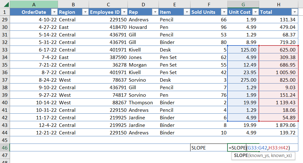
To use the slope function in Excel, you need to have two sets of coordinates that represent the points on the line. These coordinates can be in the form of (x,y) pairs, or they can be two columns of data with one representing the x-values and the other representing the y-values. Once you have your data ready, you can use the slope function by typing “=SLOPE(array1,array2)” into a cell, where “array1” and “array2” are the ranges of cells containing your data.

The slope function returns a value that represents the slope of the line in relation to the x-axis. A positive value indicates that the line is sloping upward, while a negative value indicates that it is sloping downward. A value of zero means that the line is horizontal.

In addition to trend analysis, the slope function can also be useful in statistical analysis. For example, you could use it to determine the correlation between two variables, or to fit a line to a set of data points.

Overall, the slope function is an invaluable tool for working with data in Excel. Whether you’re a seasoned user or just getting started, it’s worth learning how to use this function to get the most out of your spreadsheet analysis.

=SLOPE(array1, array2)

“array1” is a range of cells containing the y-values of the data points

“array2” is a range of cells containing the x-values of the data points. Both arrays must have the same number of rows or columns.

For example, if you had data in the range A1:A10 and B1:B10, and you wanted to calculate the slope of the line formed by this data, you could use the following formula:

=SLOPE(A1:A10, B1:B10)

This would return the slope of the line formed by the data in these ranges.

Note that the slope function only works with two-dimensional data. If you have more than two variables, you will need to use a different method to calculate the slope.

1. Organize your data in a table with the x-values in one column and the y-values in another column. Make sure that the x-values and y-values are paired correctly.
2. Select the cell where you want the result of the slope function to appear.
3. Type “=SLOPE(” into the cell. Select the range of cells containing the y-values of the data points. This should be the first argument for the function. Type a comma after the first range of cells.
4. Select the range of cells containing the x-values of the data points. This should be the second argument for the function.
5. Type a closing parenthesis “)” after the second range of cells.
6. Press “Enter” to execute the function.