- Home
- Product
- Tools
- AI Data Analyst
- Excel Formula Generator
- Excel Formula Explainer
- Google Apps Script Generator
- Excel VBA Script Explainer
- AI VBA Code Generator
- Excel VBA Code Optimizer
- Excel VBA Code Debugger
- Google Sheets Formula Generator
- Google Apps Script Explainer
- Google Sheets Formula Explainer
- Google Apps Script Optimizer
- Google Apps Script Debugger
- AI Excel Spreadsheet Generator
- AI Excel Assistant
- AI Graph Generator
- Pricing
What is IFERROR Function in Excel?
The IFERROR function in Excel checks for errors in a formula and returns a custom result if an error is found. This function is useful for hiding errors that occur in formulas, making the results of the formula easier to read and interpret.
Description
The IFERROR function in Excel traps and handles errors in a formula. It tests a specified expression and if an error is found, it returns a specified value.
This function is helpful in avoiding errors in a formula and provides an alternative solution in case of an error.
The syntax for this function is IFERROR(value, value_if_error). The first argument is the value or expression to be tested and the second argument is the value that should be returned in case of an error.
This function can be used in various formulas and is especially helpful in nested formulas.
Struggling with your Excel formulas?
Looking for a faster and easier way to write Excel formulas? Try AI Excel Formula Generator and turn your text into formulas with just a few clicks.
Syntax
=IFERROR(value, value_if_error)
Where “value” is the value or formula that you want to test for an error, and “value_if_error” is the value that you want to display if an error occurs.
For example:
=IFERROR(A1/B1, “Error”)
This formula divides the value in cell A1 by the value in cell B1 and returns the result. If an error occurs (e.g. division by zero), it returns the text “Error” instead of the error message.
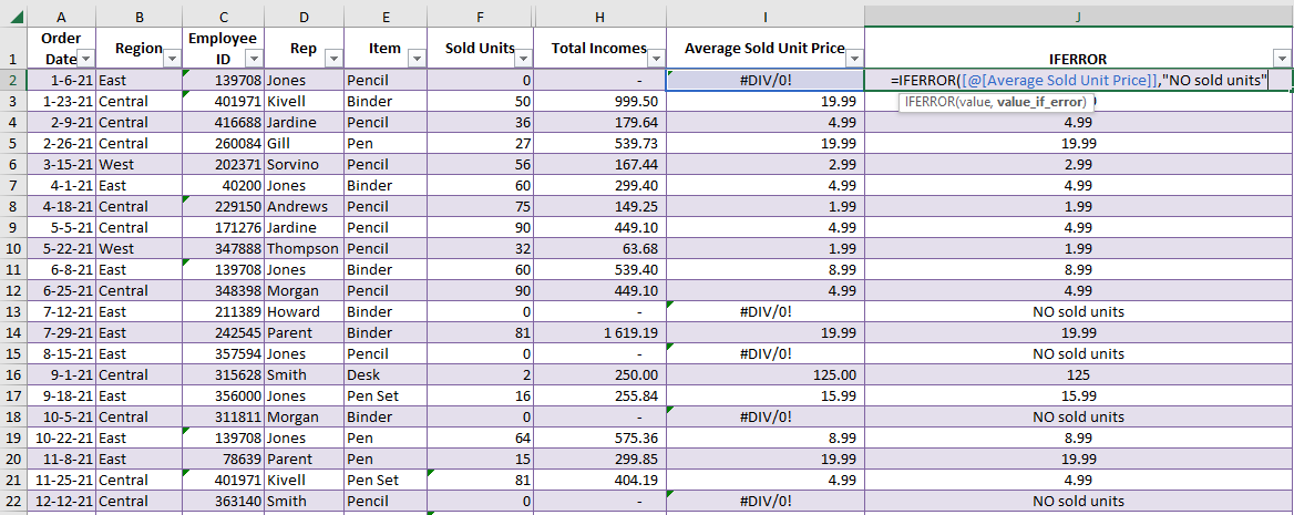
As you can see in the example below, iferror formula returns the value if there’s an error in column I. However, column I calculates the average sold units price, and if sold units are 0 that means we need more sales and error pups up.
How to use IFERROR function MS Excel in your workbook:

- Open a new or existing Excel worksheet.
- In the cell where you want to display the result of the IFERROR function, type “=IFERROR(“
- Enter the value or formula that you want to test for an error. For example, if you want to test the formula “=A1/B1” for an error, you would enter “=IFERROR(A1/B1,”
- Enter the value that you want to display if an error occurs. This can be a number, text, or a reference to a cell. For example, if you want to display the text “Error” if an error occurs, you would enter “=IFERROR(A1/B1,”Error”)”
- Press enter or click the checkmark to complete the formula.
- Repeat the formula in the cells you want to apply it.
- If the formula doesn’t produce an error the result will be the result of the formula, in case of an error it will show the value that you entered in the value_if_error argument.
- You can also use it in combination with other functions to make a complex formula that checks for an error before performing a calculation.
Note: Keep in mind that this function only works with the most common error types such as #DIV/0! #N/A, #NAME?, #NULL!, #NUM!, #REF! and #VALUE!.
Frequently Asked Questions
The IFERROR formula can handle a variety of errors, including #N/A, #VALUE!, #REF!, #DIV/0!, #NUM!, and #NAME? errors.
The IFERROR formula evaluates the value argument and checks for errors. If no errors occur, the function returns the result of the value argument. If an error occurs, the function returns the value specified in the value_if_error argument.
Yes, the IFERROR can be used with any formula or function in Excel that might return an error.
Read latest blog articles about Excel
WEEKLY BLOG ARTICLES WITH INDUSTRY NEWS AND HELPFUL GUIDES

7 Productivity Tools and AI Plugins for Excel
Written by Signe on . Posted in excel

Automation Tools for Excel in 2026: Built-In & Third-Party
Written by Signe on . Posted in excel

