- Home
- Product
- Tools
- AI Data Analyst
- Excel Formula Generator
- Excel Formula Explainer
- Google Apps Script Generator
- Excel VBA Script Explainer
- AI VBA Code Generator
- Excel VBA Code Optimizer
- Excel VBA Code Debugger
- Google Sheets Formula Generator
- Google Apps Script Explainer
- Google Sheets Formula Explainer
- Google Apps Script Optimizer
- Google Apps Script Debugger
- AI Excel Spreadsheet Generator
- AI Excel Assistant
- AI Graph Generator
- Pricing
What is VLOOKUP function in Excel?
The VLOOKUP function in Excel is used for vertical lookups. It searches for a specific value in the leftmost column of a table and returns a corresponding value from a different column in the same row.
Description
The Vlookup function MS Excel is a tool that allows users to quickly search for and retrieve information stored in a spreadsheet. It is particularly useful for quickly finding values in large datasets where manual searches would be too time-consuming.
Vlookup stands for “vertical lookup“. It allows users to search for a specific value in the leftmost column of a table and retrieve a value from the same row in a different column. This is useful in many situations, such as when you need to find a customer‘s order number based on their name or a product‘s price based on its ID.
Using the Vlookup function is simple. First, the user must select the range of cells that contains the data they want to search. Then, they enter the value they are searching for in the first argument of the function. The second argument specifies which column of the data range contains the value they are looking for. The third argument is optional and allows the user to specify what kind of search to perform. Finally, the last argument is the cell that will contain the resulting value.
A Vlookup function is an invaluable tool for quickly finding information stored in a large Excel spreadsheet. It can save users a lot of time and effort when compared to manual searches. It is also useful for quickly retrieving values from different columns in the same row, enabling users to quickly perform calculations or generate reports.
Struggling with your Excel formulas?
Looking for a faster and easier way to write Excel formulas? Try AI Excel Formula Generator and turn your text into formulas with just a few clicks.
Syntax
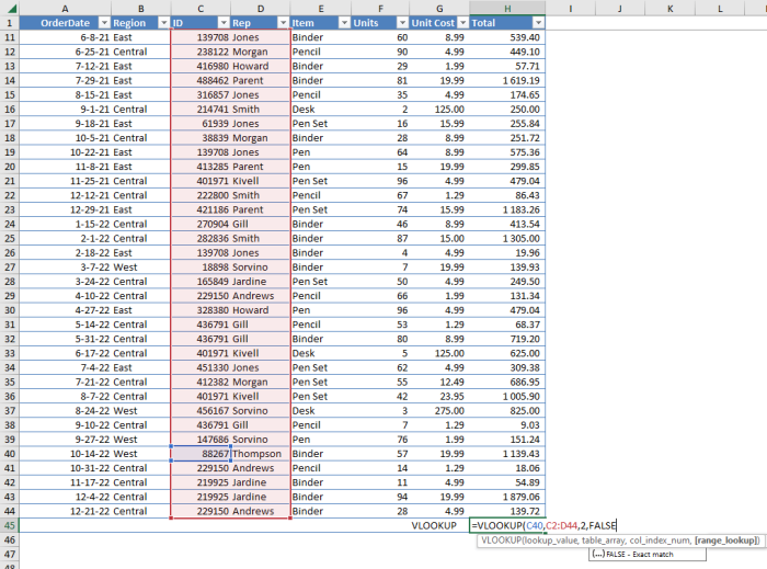
=VLOOKUP(lookup_value, table_array, col_index_num, [range_lookup])
lookup_value – The value to search for in the leftmost column of the table array.
table_array – The table array that contains the data to be searched.
col_index_num – The column number in the table array from which the matching value must be returned.
[range_lookup] – A logical value that specifies whether you want VLOOKUP to find an exact match or an approximate match:
- TRUE for an approximate match
- FALSE for an exact match.
- The default value is TRUE.

How to use VLOOKUP function in your workbook:
- Open your Excel file and select the cell that you want to display the result of the Vlookup.
- Type in the formula =VLOOKUP(.
- Enter the value that you want to search for. This is often referred to as the lookup value.
- Enter the range of cells that you want to search in. This range needs to include the column that contains the value you want to return.
- Enter the column number of the value that you want to return.
- Enter either TRUE or FALSE to indicate whether or not an exact match is required.
- Press enter to complete the formula.
- The result of the Vlookup will appear in the cell you selected.
Read latest blog articles about Excel
WEEKLY BLOG ARTICLES WITH INDUSTRY NEWS AND HELPFUL GUIDES

7 Productivity Tools and AI Plugins for Excel
Written by Signe on . Posted in excel

Automation Tools for Excel in 2026: Built-In & Third-Party
Written by Signe on . Posted in excel

