How To Sum A Column In Excel: Summation Formula

Explore other articles
- Agentic AI vs Hyperautomation: Choose the Right Automation Strategy
- Predictive Analytics in Marketing: From Data to ROI
- How To Convert Meeting Notes Into Action Items With Agentic AI
- Microsoft Copilot vs Ajelix: I Tested Both After the Agent 365 Launch
- Top 6 Google Sheets Add-ons That Will Actually Save You Time
- The EU AI Act: What Businesses Need to Do Before August 2026
- What are AI Agent Skills?
- How to Analyze SEO Data (And Do Something With It)
- How To Analyse Google Analytics Data With AI
- Ajelix Is Now Available Inside Google Workspace™
- Agentic AI in HR: Turn Raw Data Into Board-Ready Dashboard
- Ajelix Launches Agent Skills: Give Your AI Agent a Specialized Skill Set
- Ajelix Launches Text-to-Speech: Speak and Listen in 36 Languages
- AI Agent for Marketing: Use Cases & Best Platforms
- YouTube Analytics AI Dashboard & Template: Analyze Performance
- 4 Agentic AI Trends in 2026 You Must Know
- What Is AI Orchestration? A Complete Guide
- 8 Best Agentic AI Tools in 2026 (Reviewed by Our Team)
- Convert PDF To Excel Using AI: 4 Ways AI Agents Work With PDFs
- GLM-5.1. is Now Available on Ajelix AI Chat
Try AI in Excel
Mastering basic spreadsheet functions is crucial for data analysis, and one of the most fundamental is calculating sums. Whether you’re managing budgets, tracking inventory, or analyzing survey results, knowing how to sum a column in Excel is an essential skill.
TL;DR
The Excel SUM function lets you quickly total values using =SUM(range), whether the data is in one column, multiple columns, or scattered ranges. You can sum manually, use AutoSum (Σ) for a one-click total, or sum entire columns with =SUM(A:A) for dynamic updates. For non-contiguous data, list multiple ranges: =SUM(A1:A5, C1:C5, E1:E5). The fastest shortcut is Alt + =, which auto-inserts the SUM formula and guesses the range. You can also use the Excel formula generator so you can automatically create formulas from your prompts. These methods cover everything from simple totals to flexible multi-range summing.
This guide will explain the ins and outs of the summation formula and demonstrate how to efficiently total a column of numbers. We’ll cover different methods to add up a column, ensuring you can quickly and accurately calculate the sum of your data, no matter the size of your spreadsheet.
What is the SUM Function in Excel?
The SUM function in Excel adds up values across a range of cells. It can be used to sum up numbers, text, or logical values. Syntax for this formula is =SUM(number1, [number2], …)
SUM Syntax
=SUM(number1, [number2], …)
how to sum a column in Excel?
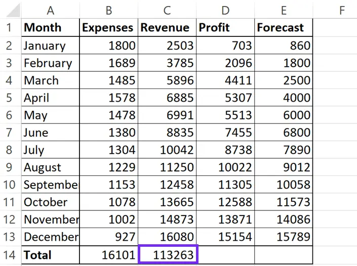
Summing a column in Excel is a fundamental skill. Whether you need to calculate totals, analyze data, or manage finances, understanding how to use the summation formula is essential.
Learn how to sum an Excel column from basic formulas to shortcuts for summing entire columns.
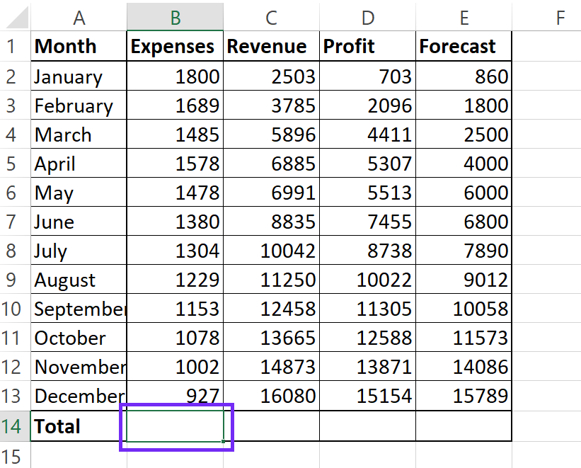
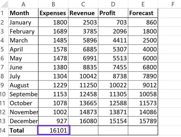
- Select the Cell
Click on the cell where you want the sum to appear. This is typically at the bottom of the column you are summing, or in a designated area for calculations.
- Enter the Formula
Type
=SUM(. Excel will automatically start suggesting functions as you type.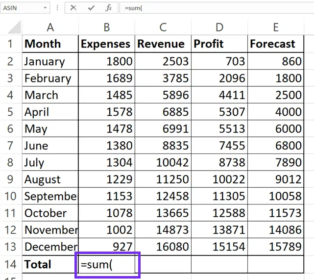
- Select the Range
Click and drag your mouse over the cells you want to add together. This will highlight the range of cells you’re including in the summation formula. Alternatively, you can manually type the cell range, for example,
A1:A10(this would sum cells A1 through A10).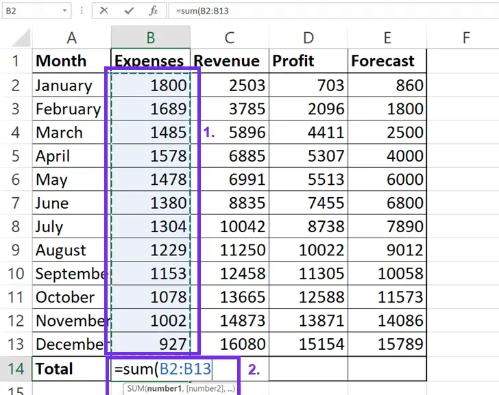
- Close the Parenthesis
Type a closing parenthesis
)to complete the formula.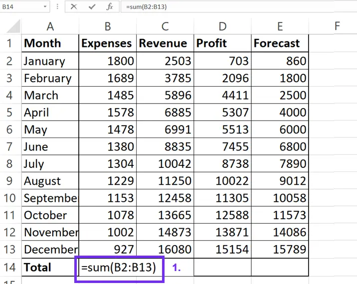
- Press Enter
Press the Enter key on your keyboard. The sum of the selected column will appear in the cell you chose.
Using the AutoSum Feature (Quick Sum Excel Column)
AutoSum offers a quick way to total a column in Excel.
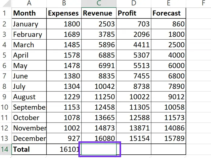
1. Select the Cell: Click on the cell below the column you want to sum (or the cell where you want the total to appear).
You might also like: SUMIF in Excel
2. Click AutoSum: On the “Home” tab of the Excel ribbon, in the “Editing” group, you’ll find the AutoSum button (it looks like a Greek sigma symbol Σ). Click it.
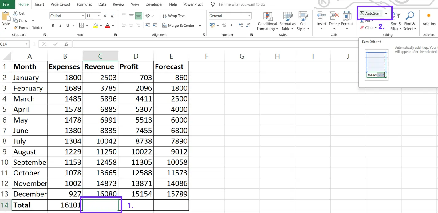
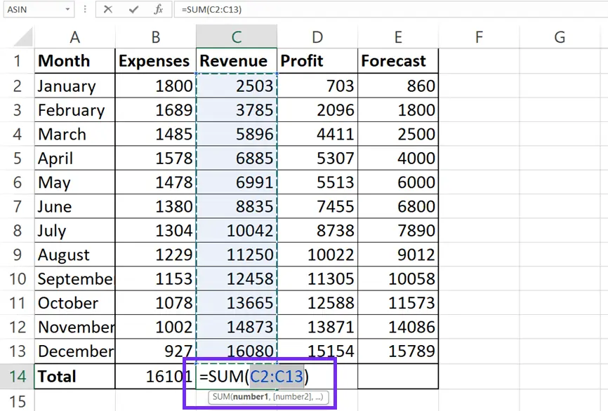
3. Verify the Range: Excel will automatically select what it thinks is the range of cells you want to sum. Double-check that the selected range is correct. If it’s not, you can adjust it by clicking and dragging over the correct cells.
You might also like: Average function in Excel
4. Press Enter: Press Enter to calculate the sum.
Summing an Entire Column (Excel Sum Entire Column)
If you want to add together a column in Excel regardless of how many rows it contains (and potentially add data to it later), you can reference the entire column.
1. Select the Cell: Choose the cell where you want the sum to be displayed.
2. Enter the Formula: Type =SUM(A:A) (replace A with the letter of the column you want to sum). This formula will sum every cell in column A.
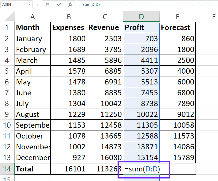
3. Press Enter: Press Enter. The sum of the entire column will be calculated. This method is particularly useful for dynamically updating totals as you add more data to the column.
You might also like: Free Profitability Index Calculator Online
Formula for Sum of Column with Non-Contiguous Data
Sometimes your data isn’t in a continuous column. You can still use the SUM formula.
1. Select the Cell: Choose the cell for the total.
2. Enter the Formula: Type =SUM(.
3. Select the Ranges: Click and drag over the first range of cells. Then, type a comma , and select the next range. Repeat this process for all the ranges you want to include. For example: =SUM(A1:A5, C1:C5, E1:E5)
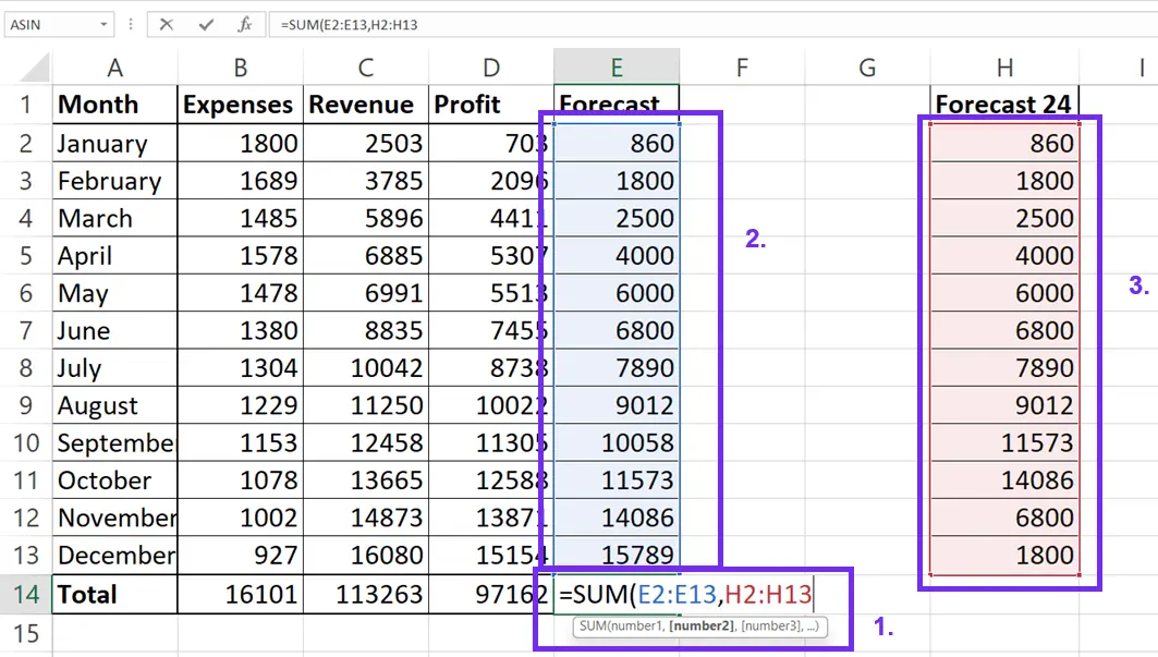
4. Close Parenthesis and Enter: Type ) and press Enter.
These methods provide you with several ways to sum a column in Excel. Whether you’re using the full summation formula, the quick AutoSum, or referencing the entire column, you can efficiently calculate the sum of your data. Remember to double-check your cell ranges to ensure accurate results.
Excel Template Download To SUM Columns
shortcut key for sUM in excel
Excel offers several shortcuts to speed up your work, and summing data is no exception. While there isn’t one single, universally recognized keyboard shortcut for sum in Excel that directly inserts the entire =SUM() formula with selected range, the most common and efficient shortcut for sum in Excel is Alt + =.
This sum shortcut Excel quickly inserts the =SUM() function and intelligently guesses the range of cells you want to sum, usually the cells directly above or to the left of the active cell.
This shortcut key for sum in Excel is a huge time-saver compared to manually typing the Excel sum formula shortcut or using the mouse to select the range. While other methods exist, this shortcut for sum is the most widely used and remembered shortcut for sum.
Conclusions
So, there you have it! Figuring out how to sum a column in Excel is a total game-changer. Whether you’re a spreadsheet newbie or a seasoned pro, knowing how to quickly total a column is super useful. If you need help with Excel formula writing you can always use the Excel formula generator or use a formula cheat sheet.
We walked through a bunch of ways to do it, from typing out the whole summation formula (like =SUM(A1:A10)) to using the handy AutoSum button. And don’t forget the shortcut key for sum in Excel – Alt + = – that’s a real time-saver!
Whether you’re summing a few cells or trying to sum an Excel entire column, these tips will help you add up a column in Excel like a boss. So go forth and conquer those spreadsheets! You’ve got this!
FAQ
You can still use the SUM formula. Enter =SUM(, then click and drag over the first range of cells, type a comma, click and drag over the next range, and so on. For example: =SUM(A1:A5, C1:C5, E1:E5).
Yes! Use the formula =SUM(A:A) (replace A with the column letter). This will sum all cells in column A, even if you add more data later. The sum will automatically update.
This requires more advanced functions like SUMIF or SUMIFS. SUMIF allows you to sum cells based on one criterion, while SUMIFS allows for multiple criteria. Look up these functions in Excel’s help for more details.
Yes, you can! You can either use the SUM function and include multiple ranges (e.g., =SUM(A1:A10, C1:C10)) or sum each column individually and then sum those totals.
Speed up your spreadsheet tasks with Ajelix AI in Excel